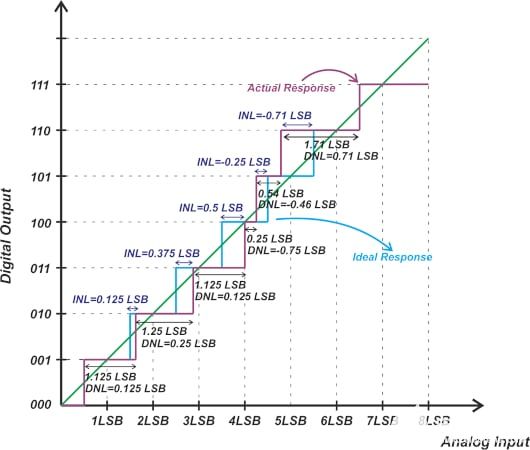
Abstract: To understand the effects of integral non-linearity errors, the most straightforward approach is to analyze a simple sine wave and apply well-known trigonometric identities to a non-ideal, analog-to-digital output transfer function, which contains an INL error.
With an ideal system, a single-tone sine wave with amplitude A and frequency fo,
X(t) = Asin(2π fot)
Sampling with an ADC with a period of T results in a discrete signal:
X[n]=Asin(2π fonT),
where X[n] is the discrete-time signal obtained from the uniform sampling of X(t) every T seconds. The reciprocal 1/T = F is called the sampling rate or sampling frequency.
A particularly important class of systems consists of those that are linear and time invariant, or "LTI." These two properties in combination lead to especially convenient representations for such systems. Most important, the relationship between the input to a LTI system X[n] and the output Y[n] can be given by a convolution sum. Convolution is fundamental to the analysis and description of LTI systems. In this example, we will only be analyzing the linearity of a system.
A linear system is one that satisfies the superposition principle. Simply stated, the principle of superposition requires that the response of the system to a weighted sum of signals be equal to the corresponding weighted sum of the responses (outputs) of the system to each individual input signals. The superposition property greatly simplifies the analysis of linear systems. Because of the decomposition property, you can evaluate separately the different components of the output.
Comparing an ideal ADC transfer curve to a transfer curve with an INL error, it is easy to demonstrate how a system with INL error yields a non-linear output. The output Y3[n] is not equal to the sum of output Y1[n] +Y2[n] when its input is X3[n] = X1[n] + X2[n]. More precisely, F(X1 + X2) ≠ F(X1) + F(X2). As a result, the non-linearity error produces additional, unwanted, internally generated sinusoids which can increase the design cost and the filter complexity. (Electrical engineers recognize this effect of internally generated sinusoids as intermodulation distortion.)
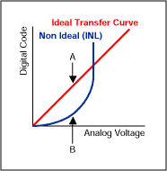
Figure 1. The distance between the tip of arrow A and the tip of arrow B, is a measurement of the INL error.
In the above figure, the ideal transfer function is draw as a straight linear line. In this example, the non ideal transfer curve, which includes INL error, is drawn just as a second order function Y[n] = k[X[n]]^2. In reality, the non ideal transfer function may also contain second order, third order, fourth order, etc., components Y[n] = kX1[n] + k2X[n]^2 + k3X[n]^3 + k4X[n]^4 + ...
For the following analysis, only the second order component is considered.
X1[n] = sin(2π × fo × nT) fo = 1Hz (separated out fo for clarity), amplitude A=1, no phase
Y1[n] = kX1[n]X1[n] set constant k = 1 for simplicity in this example
Y1[n] = sin(2π × 1 × nT)sin(2π × 1 × nT)
Note: Recall from trigonometry identities, Sin(A)Sin(B) = Cos(A-B)/2 - Cos(A+B)/2
Y1[n] = cos(2π × 1 × nT - 2π × 1 × nT)/2 - cos(2π × 1 × nT + 2π × 1 × nT)/2
Y1[n] = cos(0)/2 - cos(4π × 1 × nT)/2
Y1[n] = 1/2 - cos(2π × 2 × nT)/2 (cosine wave with fo = 2Hz and peak amplitude of -0.5)
![Figure 2. Y2[n] = X2[n]2 = 1/2 - cos(2pie x 6 x nT)/2.](/article/UploadPic/2009-5/20095711455381.gif)
Figure 2. Y2[n] = X2[n]2 = 1/2 - cos(2π × 6 × nT)/2.
X2[n] = sin(2π × fo × nT) with fo = 3Hz with an amplitude A=1
Y2[n] = sin(2π × 3 × nT)sin(2π × 3 × nT)
Y2[n] = cos(2π × 3 × nT - 2π × 3 × nT)/2 - cos(2π × 3 × nT + 2π × 3 × nT)/2
Y2[n] = cos(0)/2 - cos(4π × 3 × nT)/2
Y2[n] = 1/2 - cos(2π × 6 × nT)/2 (cosine wave with fo = 6Hz and peak amplitude of -0.5)
![Figure 3. Y1[n] = X1[n]2 = 1/2 - cos(2pie x 2 x nT)/2.](/article/UploadPic/2009-5/20095711457936.gif)
Figure 3. Y1[n] = X1[n]2 = 1/2 - cos(2π × 2 × nT)/2.
We can now apply X3[n] = X1[n] + X2[n] , with Y3[n] = [X[3]]^2
Y3[n] = [ X1[n] + X2[n] ]^2
Y3[n] = X1[n]X1[n] + 2 X1[n]X2[n] + X2[n]X2[n]
As previously noted:
X1[n]X1[n] results in a constant value of 1/2 and a cosine wave of 2Hz, amplitude -0.5
X2[n]X2[n] results in a constant value of 1/2 and a cosine wave of 6Hz, amplitude -0.5
Therefore,
![Figure 4. Y3[n] = X1[n]^2 = 1 - cos(2pie x 2 x nT)/2 - cos(2pie x 6 x nT)/2.](/article/UploadPic/2009-5/20095711459688.gif)
Figure 4. Y3[n] = X1[n]^2 = 1 - cos(2π × 2 × nT)/2 - cos(2π × 6 × nT)/2.
However,
![Figure 5. Y3[n] = X1[n] + X2[n])^2 = 1 - cos(2pie x 2 x nT)/2 - cos(2pie 6 x nT)/2 + cos(2pie x 4 x nT).](/article/UploadPic/2009-5/200957114511317.gif)
Figure 5. Y3[n] = X1[n] + X2[n])^2 = 1 - cos(2π × 2 × nT)/2 - cos(2π × 6 × nT)/2 + cos(2π × 4 × nT).
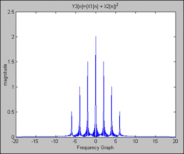
As a result of the integral non-linearity error, we have added two additional cosine waves of 2Hz and 4Hz. The superposition principle is not satisfied, therefore the system is non-linear and is not a Linear Time Invariant system. As noted above, filtering needs to be applied to suppress the additional unwanted frequencies (or side lobes), adding design complexity and cost.
% Maxim Integrated Products
% Magnitude Verses Frequency Plots - Non-Linearity Error
n = 0:1023;
w0 = 0.02*pi; % w0 = 2*pi*1*0.01 , frequency = 1Hz, Sample period = .01s
w1 = 0.06*pi; % w1 = 2*pi*3*0.01 , frequency = 3Hz, Sample period = .01s
N = 2048;
w = (-N/2:(N-1)/2)*2*pi/N;
x1=cos(w0*n); % X1[n] = cos(2*pi*1*n*0.01) freq = 1Hz , Sample period = .01s
x2=cos(w1*n); % X2[n] = cos(2*pi*3*n*0.01) freq = 3Hz , Sample period = .01s
x3=x1+x2;
y1=x1.*x1; % Y1[n] = [X1[n]]^2
y2=x2.*x2; % Y2[n] = [X2[n]]^2
y3=y1+y2;
y4=x3.*x3;
L = 1024;
Z0=[y1(1:L) zeros(1, 2048 - L)];
Z1=[y2(1:L) zeros(1, 2048 - L)];
Z2=[y3(1:L) zeros(1, 2048 - L)];
Z3=[y4(1:L) zeros(1, 2048 - L)];
%Perform FFT on signals
Z5=fft(Z0, N);
fftshift(Z5);
Z6=fft(Z1, N);
fftshift(Z6);
Z7=fft(Z2, N);
fftshift(Z7);
Z8=fft(Z3, N);
fftshift(Z8);
%Plot signals
subplot(2,2,1);plot(w/(.02*pi),abs(fftshift(Z5)/512)), xlabel(''), ylabel('magnitude');
title('X1[n]^2');
subplot(2,2,2);plot(w/(.02*pi),abs(fftshift(Z6)/512)), xlabel(''), ylabel('magnitude');
title('X2[n]^2');
subplot(2,2,3);plot(w/(.02*pi),abs(fftshift(Z7)/512)), xlabel('Frequency Graph'), ylabel('magnitude');
title('Y3[n]=X1[n]^2 + X2[n]^2');
subplot(2,2,4);plot(w/(.02*pi),abs(fftshift(Z8)/512)), xlabel('Frequency Graph'), ylabel('magnitude');
title('Y3[n]=(X1[n] + X2[n])^2');
With an ideal system, a single-tone sine wave with amplitude A and frequency fo,
X(t) = Asin(2π fot)
Sampling with an ADC with a period of T results in a discrete signal:
X[n]=Asin(2π fonT),
where X[n] is the discrete-time signal obtained from the uniform sampling of X(t) every T seconds. The reciprocal 1/T = F is called the sampling rate or sampling frequency.
A particularly important class of systems consists of those that are linear and time invariant, or "LTI." These two properties in combination lead to especially convenient representations for such systems. Most important, the relationship between the input to a LTI system X[n] and the output Y[n] can be given by a convolution sum. Convolution is fundamental to the analysis and description of LTI systems. In this example, we will only be analyzing the linearity of a system.
A linear system is one that satisfies the superposition principle. Simply stated, the principle of superposition requires that the response of the system to a weighted sum of signals be equal to the corresponding weighted sum of the responses (outputs) of the system to each individual input signals. The superposition property greatly simplifies the analysis of linear systems. Because of the decomposition property, you can evaluate separately the different components of the output.
Comparing an ideal ADC transfer curve to a transfer curve with an INL error, it is easy to demonstrate how a system with INL error yields a non-linear output. The output Y3[n] is not equal to the sum of output Y1[n] +Y2[n] when its input is X3[n] = X1[n] + X2[n]. More precisely, F(X1 + X2) ≠ F(X1) + F(X2). As a result, the non-linearity error produces additional, unwanted, internally generated sinusoids which can increase the design cost and the filter complexity. (Electrical engineers recognize this effect of internally generated sinusoids as intermodulation distortion.)

Figure 1. The distance between the tip of arrow A and the tip of arrow B, is a measurement of the INL error.
In the above figure, the ideal transfer function is draw as a straight linear line. In this example, the non ideal transfer curve, which includes INL error, is drawn just as a second order function Y[n] = k[X[n]]^2. In reality, the non ideal transfer function may also contain second order, third order, fourth order, etc., components Y[n] = kX1[n] + k2X[n]^2 + k3X[n]^3 + k4X[n]^4 + ...
For the following analysis, only the second order component is considered.
X1[n] = sin(2π × fo × nT) fo = 1Hz (separated out fo for clarity), amplitude A=1, no phase
Y1[n] = kX1[n]X1[n] set constant k = 1 for simplicity in this example
Y1[n] = sin(2π × 1 × nT)sin(2π × 1 × nT)
Note: Recall from trigonometry identities, Sin(A)Sin(B) = Cos(A-B)/2 - Cos(A+B)/2
Y1[n] = cos(2π × 1 × nT - 2π × 1 × nT)/2 - cos(2π × 1 × nT + 2π × 1 × nT)/2
Y1[n] = cos(0)/2 - cos(4π × 1 × nT)/2
Y1[n] = 1/2 - cos(2π × 2 × nT)/2 (cosine wave with fo = 2Hz and peak amplitude of -0.5)
![Figure 2. Y2[n] = X2[n]2 = 1/2 - cos(2pie x 6 x nT)/2.](/article/UploadPic/2009-5/20095711455381.gif)
Figure 2. Y2[n] = X2[n]2 = 1/2 - cos(2π × 6 × nT)/2.
X2[n] = sin(2π × fo × nT) with fo = 3Hz with an amplitude A=1
Y2[n] = sin(2π × 3 × nT)sin(2π × 3 × nT)
Y2[n] = cos(2π × 3 × nT - 2π × 3 × nT)/2 - cos(2π × 3 × nT + 2π × 3 × nT)/2
Y2[n] = cos(0)/2 - cos(4π × 3 × nT)/2
Y2[n] = 1/2 - cos(2π × 6 × nT)/2 (cosine wave with fo = 6Hz and peak amplitude of -0.5)
![Figure 3. Y1[n] = X1[n]2 = 1/2 - cos(2pie x 2 x nT)/2.](/article/UploadPic/2009-5/20095711457936.gif)
Figure 3. Y1[n] = X1[n]2 = 1/2 - cos(2π × 2 × nT)/2.
We can now apply X3[n] = X1[n] + X2[n] , with Y3[n] = [X[3]]^2
Y3[n] = [ X1[n] + X2[n] ]^2
Y3[n] = X1[n]X1[n] + 2 X1[n]X2[n] + X2[n]X2[n]
As previously noted:
X1[n]X1[n] results in a constant value of 1/2 and a cosine wave of 2Hz, amplitude -0.5
X2[n]X2[n] results in a constant value of 1/2 and a cosine wave of 6Hz, amplitude -0.5
| For 2X1[n]X2[n] | = 2sin(2π × 1 × nT)sin(2π × 3 × nT) |
| = cos(2π × 1 × nT - 2π × 3 × nT) - cos(2π × 1 × nT + 2π × 3 × nT) | |
| = cos(-4π × nT) - cos(8π × nT) | |
| = cos(-2π × 2 × nT) - cos(2π × 4 × nT) | |
| = cos(2π × 2 × nT) - cos(2π × 4 × nT) (cosine waves of 2Hz and 4Hz) |
Therefore,
| For Y3[n] | = X1[n]^2 + X2[n]^2 |
| = Y1[n] + Y2[n] | |
| = 1 - cos(2π × 2 × nT)/2 - cos(2π × 6 × nT)/2 |
![Figure 4. Y3[n] = X1[n]^2 = 1 - cos(2pie x 2 x nT)/2 - cos(2pie x 6 x nT)/2.](/article/UploadPic/2009-5/20095711459688.gif)
Figure 4. Y3[n] = X1[n]^2 = 1 - cos(2π × 2 × nT)/2 - cos(2π × 6 × nT)/2.
However,
| For Y3[n] | = ( X1[n] + X2[n] )^2 |
| = 1 - cos(2π × 2 × nT)/2 - cos(2π × 6 × nT)/2 + cos(2π × 2 × nT) - cos(2π × 4 × nT) |
![Figure 5. Y3[n] = X1[n] + X2[n])^2 = 1 - cos(2pie x 2 x nT)/2 - cos(2pie 6 x nT)/2 + cos(2pie x 4 x nT).](/article/UploadPic/2009-5/200957114511317.gif)
Figure 5. Y3[n] = X1[n] + X2[n])^2 = 1 - cos(2π × 2 × nT)/2 - cos(2π × 6 × nT)/2 + cos(2π × 4 × nT).
As a result of the integral non-linearity error, we have added two additional cosine waves of 2Hz and 4Hz. The superposition principle is not satisfied, therefore the system is non-linear and is not a Linear Time Invariant system. As noted above, filtering needs to be applied to suppress the additional unwanted frequencies (or side lobes), adding design complexity and cost.
Listing 1: Matlab Code
% Frequency Resolution Demonstration% Maxim Integrated Products
% Magnitude Verses Frequency Plots - Non-Linearity Error
n = 0:1023;
w0 = 0.02*pi; % w0 = 2*pi*1*0.01 , frequency = 1Hz, Sample period = .01s
w1 = 0.06*pi; % w1 = 2*pi*3*0.01 , frequency = 3Hz, Sample period = .01s
N = 2048;
w = (-N/2:(N-1)/2)*2*pi/N;
x1=cos(w0*n); % X1[n] = cos(2*pi*1*n*0.01) freq = 1Hz , Sample period = .01s
x2=cos(w1*n); % X2[n] = cos(2*pi*3*n*0.01) freq = 3Hz , Sample period = .01s
x3=x1+x2;
y1=x1.*x1; % Y1[n] = [X1[n]]^2
y2=x2.*x2; % Y2[n] = [X2[n]]^2
y3=y1+y2;
y4=x3.*x3;
L = 1024;
Z0=[y1(1:L) zeros(1, 2048 - L)];
Z1=[y2(1:L) zeros(1, 2048 - L)];
Z2=[y3(1:L) zeros(1, 2048 - L)];
Z3=[y4(1:L) zeros(1, 2048 - L)];
%Perform FFT on signals
Z5=fft(Z0, N);
fftshift(Z5);
Z6=fft(Z1, N);
fftshift(Z6);
Z7=fft(Z2, N);
fftshift(Z7);
Z8=fft(Z3, N);
fftshift(Z8);
%Plot signals
subplot(2,2,1);plot(w/(.02*pi),abs(fftshift(Z5)/512)), xlabel(''), ylabel('magnitude');
title('X1[n]^2');
subplot(2,2,2);plot(w/(.02*pi),abs(fftshift(Z6)/512)), xlabel(''), ylabel('magnitude');
title('X2[n]^2');
subplot(2,2,3);plot(w/(.02*pi),abs(fftshift(Z7)/512)), xlabel('Frequency Graph'), ylabel('magnitude');
title('Y3[n]=X1[n]^2 + X2[n]^2');
subplot(2,2,4);plot(w/(.02*pi),abs(fftshift(Z8)/512)), xlabel('Frequency Graph'), ylabel('magnitude');
title('Y3[n]=(X1[n] + X2[n])^2');
References
- Discrete-Time Signal Processing, Alan Oppenheim and Ronald Schafer
- Understanding Digital Signal Processing, Richard Lyons
- Digital Signal Processing, John Proakis and Dimitris Manolakis
- Signal Processing & Linear Systems, B.P. Lathi
 電子發燒友App









評論